Welcome to the Renegade Weblog
Renegade is a pioneering Internet blogger seamlessly merging creative art and technical expertise to redefine blogging excellence.

Blog Posts
-
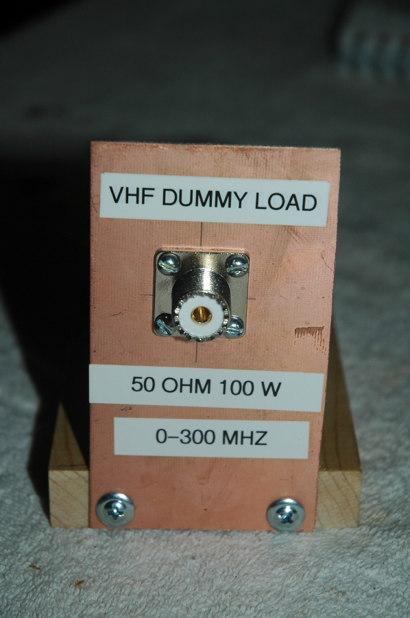
VHF 50-Ohm Dummy Load – $10
Category: Amateur Radio -
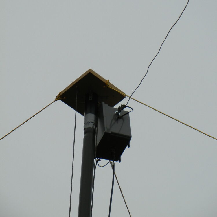
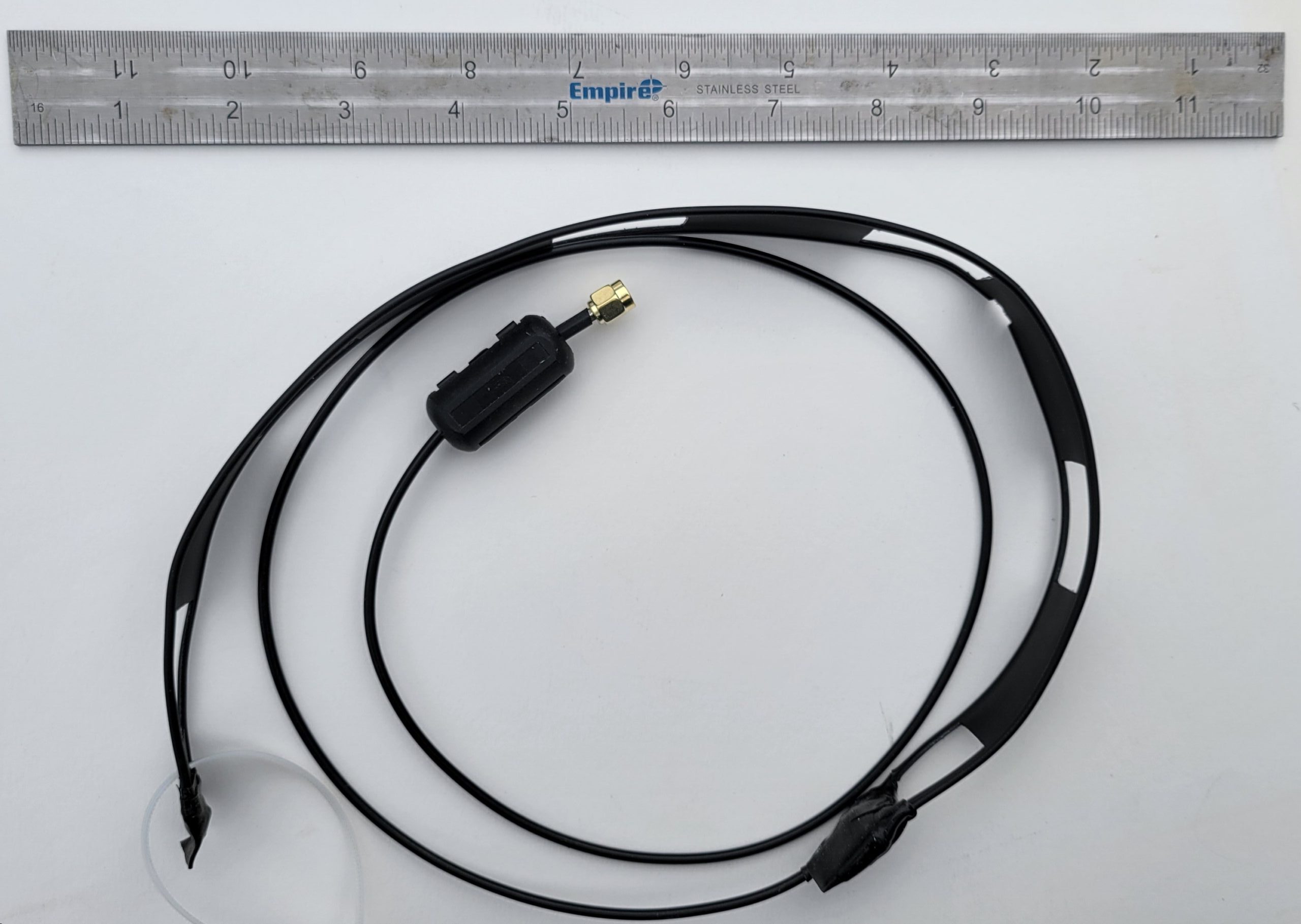
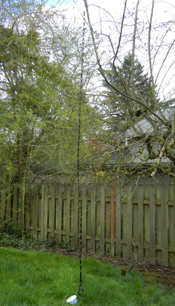
OCF HF Dipole Antenna
Category: Amateur Radio -
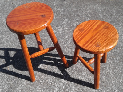
Stanton 3-Legged Stool
Category: Woodworking -
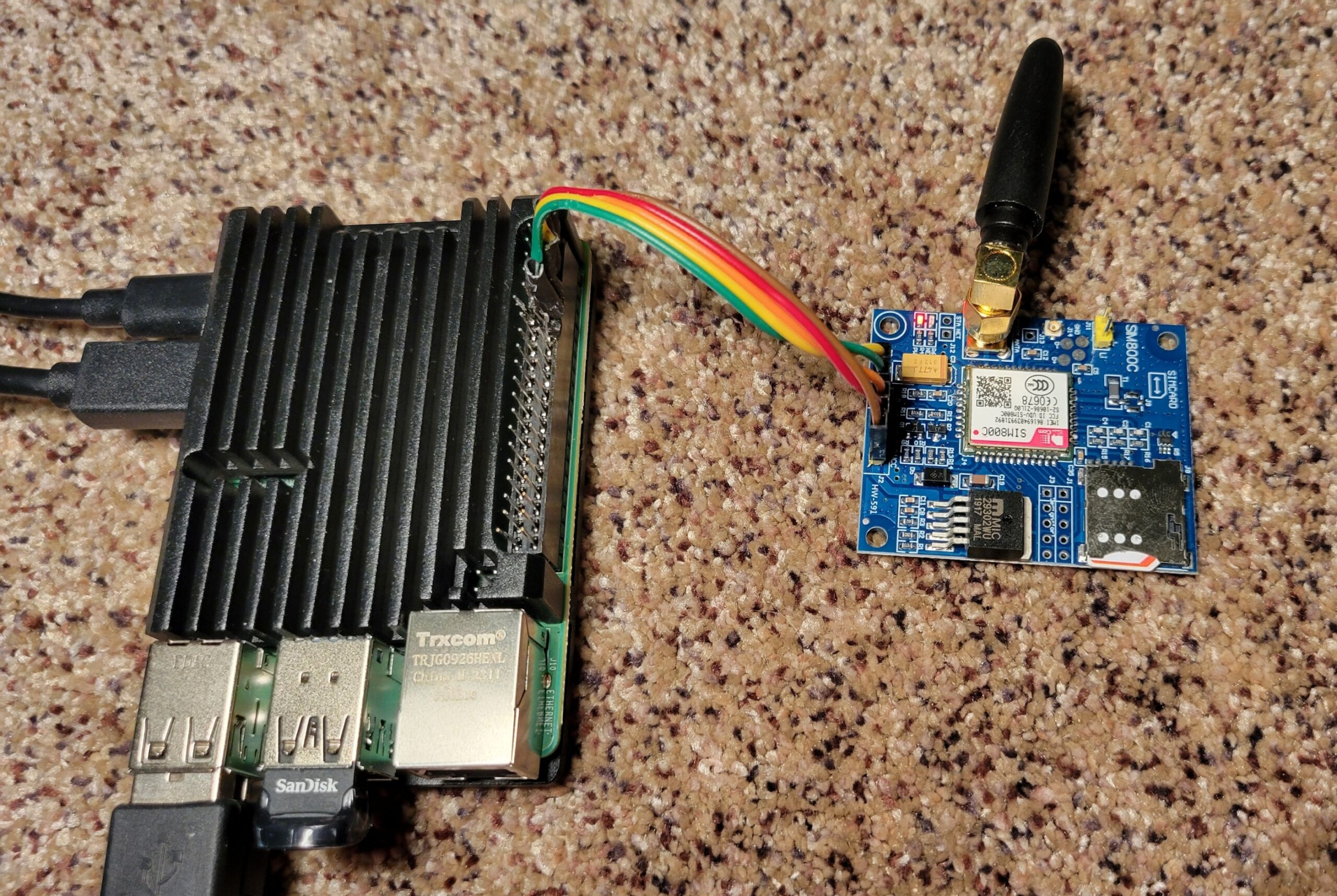
Automated (SMS) Text Messaging
Category: Computers -
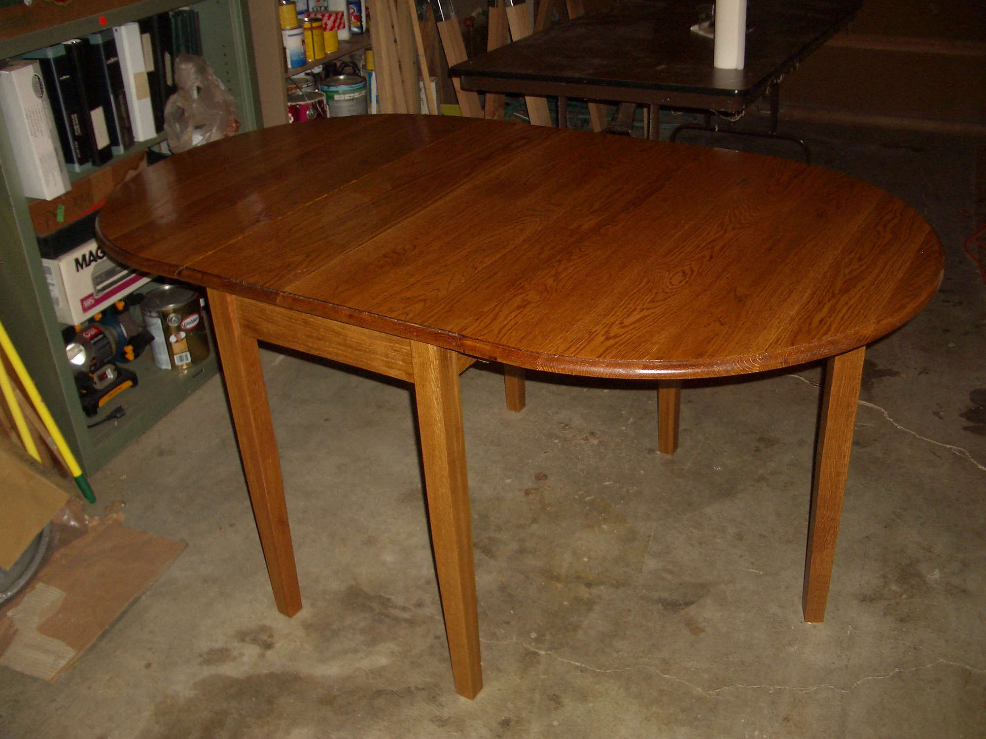
Gate Leg Drop Leaf Oak Table
Category: Woodworking -
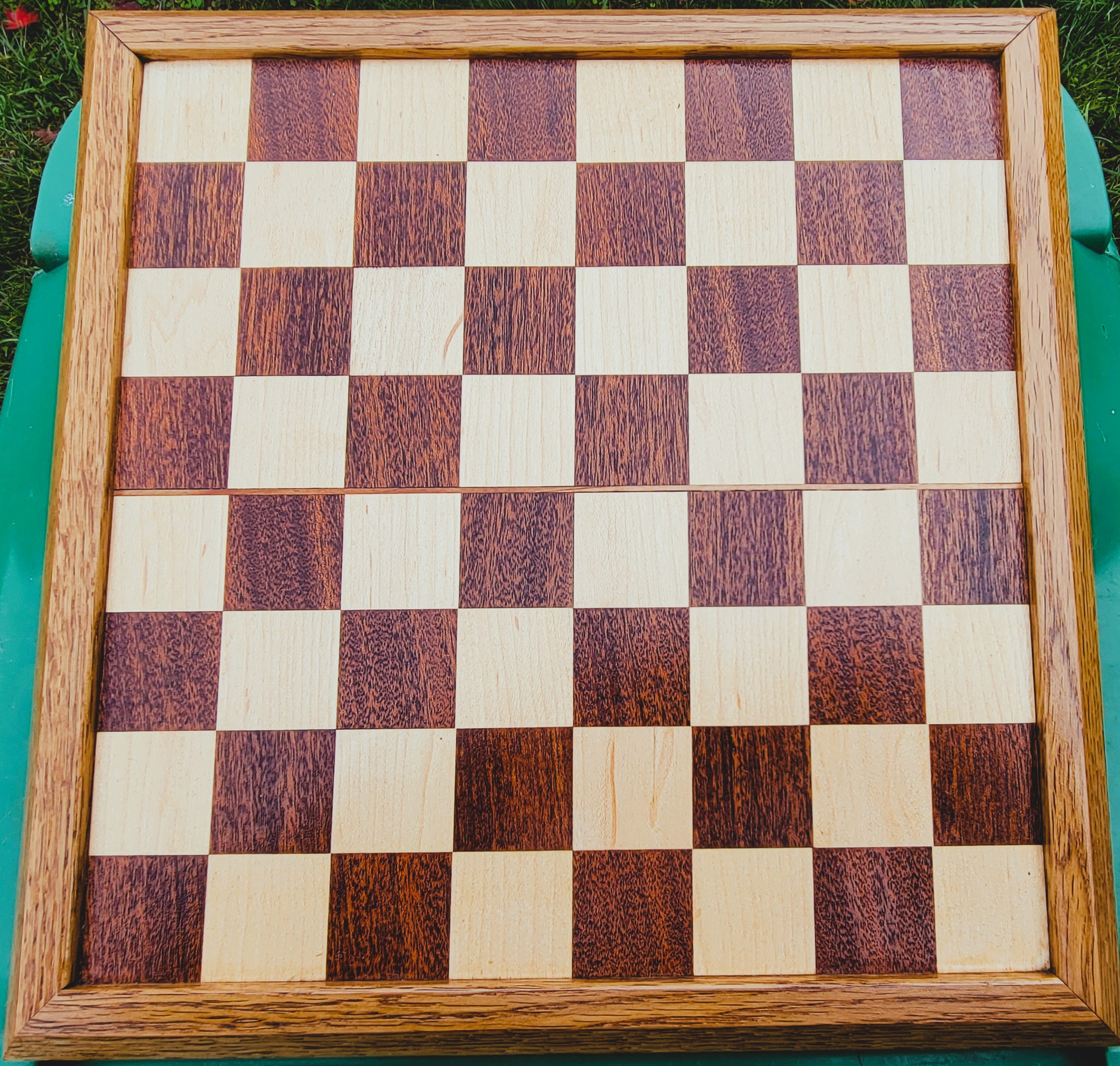
Homemade Wooden Chessboard
Category: Woodworking

Category List
- Amateur Radio (5)
- Computers (1)
- Uncategorized (1)
- Woodworking (4)