Category: Amateur Radio
-
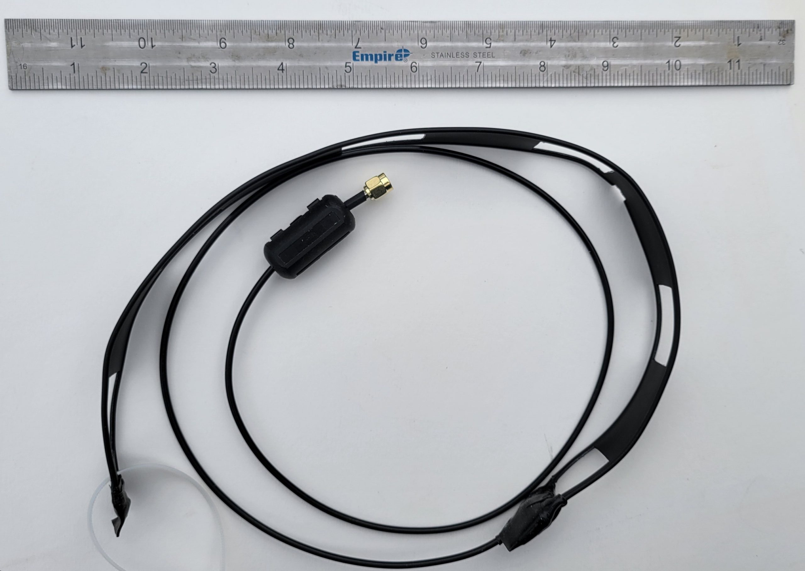
DIY UHF Slim Jim Ladder Line Antenna
Build a high-performance Amateur Radio UHF Slim Jim antenna for little or no cost using scrap materials and a few common hand tools.
-
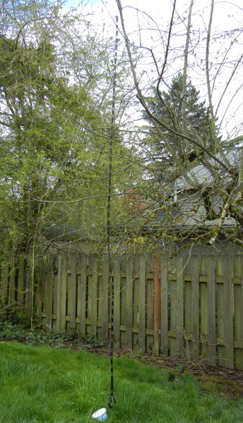
DIY 6 Meter Slim Jim Ladder Line Antenna
If you’re an Amateur Radio operator and enjoy designing and building your own antennas, like I do. This 6m Slim Jim antenna is a very gratifying project, and cheap too. The 6 Meter Ham band covers 50-51 MHz. Using an online Slim Jim calculator to get the proper dimensions, assume the Velocity Factor (Vf) =…
-
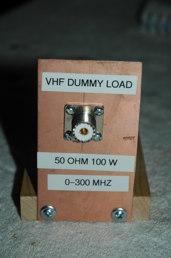
VHF 50-Ohm Dummy Load – $10
A VHF 50-ohm Dummy Load is a basic test and measurement tool for developing high frequency radio transmitters, feedlines and antennas. Not all resistors are created equal and high frequency parasitic inductance and capacitance can distort your RF measurements. Build an inexpensive VHF 50-ohm Dummy Load from a BeO (BerylliumOxide) resistor and some scrap shop…
-
OCF HF Dipole Antenna
As an Amateur Radio Enthusiast, I take great pride in designing and building my own antennas. This OCR HF Dipole Antenna is 69 ft. end-to-end in length and designed to work on the 40-20-15-10 amateur bands. When fed from 50-ohm feedline coax, a 4:1 Quanella Current Balun makes it a true balanced antenna. It is…
-
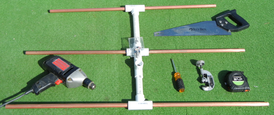
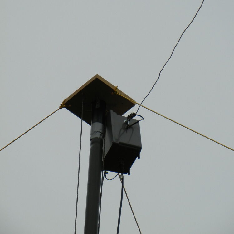
DIY Dual Band VHF/UHF Yagi Antenna
Build this high-performance DIY Dual Band VHF/UHF Yagi antenna using the simple hand tools pictured above. Low-cost PVC pipe fixtures and 1/2″ copper pipe materials are available from your local home improvement store. This was a very gratifying Ham Radio project. Actual performance exceeded simulated expectations. EZNEC simulation shows a forward gain of 12 dBi…