Arduino PID Temperature Control

Arduino PID Temperature Control
Running PID Unit

Being a dedicated nerd, I’m always fascinated by Proportional Integral Derivative (PID) process control. So when a local farmer asked me to automate a vegetable canning process, I took it as a challenge to physically realize a PID temperature control device. Of course many fine industrial controllers already exist, say from Omega, but I’d already done that so I strived to do it smaller, cheaper. The Arduino product line provides inexpensive hardware for the home Maker. Also, the Arduino development environment is easy to install and remarkably easy to use. For this reason, I decided to build an Arduino PID Temperature Control unit.

Arduino PID Temperature Control
PID Temperature Sampling

About PID
The PID process control method is well researched and commonly applied in modern industry. PID mathematics can be complicated, but (within limits) PID can compensate for thermal resistance and thermal capacitance in a system for precise temperature control. Ideal PID temperature control assumes both a heating and cooling source (with same linear thermal forcing gain). This can be difficult to achieve practically due to different heat/cool technologies. Under-sampling temperature frequently will also increase errors. There are many ways to go wrong. Even when operating correctly, wild oscillations in temperature are possible. Nevertheless PID control can be adapted to many situations.

Many PID controllers claim to autotune the Kp, Ki, Kd PID coefficients to achieve optimal performance. But I suspect these methods are often home-grown and apply only to a narrow set of conditions. PID mathematics is very complicated. Fortunately there are practical manual methods and online simulations to aid in setting these important PID parameters.

For this controller, the PID proportional output uses Pulse Width Modulation(PWM) on 2 pins. Often PWM is used to create a (time-averaged) variable DC voltage, but here the digital signal duty-cycle modulates a SSR power cycle. One pin outputs the plus(+) and a second pin the minus(-) PID output. The PWM resolution for this microcontroller is 8 bits (0-255 values) for each pin.
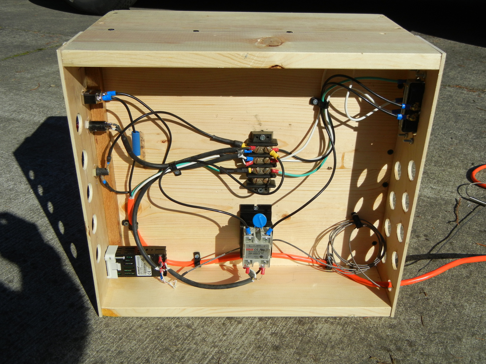
Simplified Circuit Diagram

Hardware
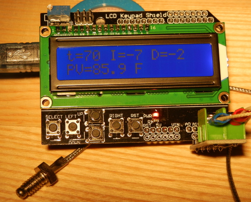
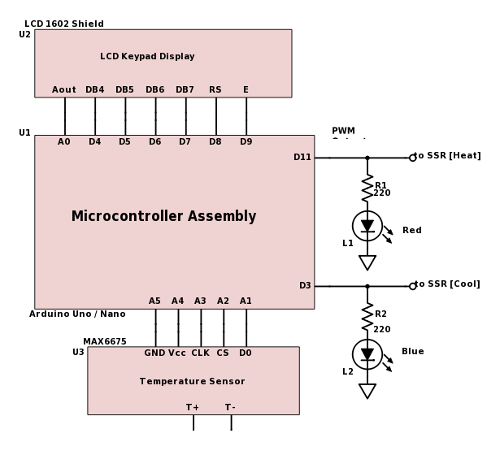
This PID controller device is composed of 3 sub-units (Arduino Uno R3, MAX6675 thermocouple temperature sensor, 1602 LCD keypad display).  An Arduino Nano and breadboard was used for testing purposes. Online cost for these units is about $11 + $5 + $4 = $20. Analog pins A1-A5 were converted to digital function for temperature sensor  power and communication. Fortunately this leaves digital pins 3, 11 (both on 16 bit TIMER2) to use for PWM modulation outputs.

Program Features
Using the LCD Keypad Display it would be possible to control every function but this is beyond the project’s scope. So the best way to experiment is through the Arduino IDE environment.

  • PID output range has units of degrees per sample period . It’s very important to set min/max PID limits for actual physical temperature forcing capability. For example, in a heat-only system the negative PID output is theoretically zero, or perhaps slightly negative (-2 degrees/minute maybe) for an ambient cooling system.
  • An over/under temperature Alarm is programmed to terminate execution immediately if min/max temperature limits are exceeded.
  • If either +/- PID output limit is reached an error is displayed on the LCD screen. While not fatal, this should be a clue that K coefficients may need adjusting.
  • The Arduino Serial Monitor tool displays PID data in progress
  • Commenting one line of code switches between PID simulation and live operation

SSR and PWM Problem
A Solid State Relay (SSR) is capable of switching on/off a 120V heavy load. But, like electromechanical relays, the switching speed is slow.  Because common, low-cost SSRs use a TRIAC Thyrister element, the power is not actually switched until the voltage phase of AC power crosses zero. The zero-crossing effect is shown in graphic below.

zero-crossing timing diagram

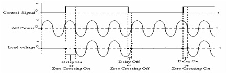
At a frequency of 60Hz the maximum delay is 1/2 cycle or 8.33ms. Considering that our PWM duty-cycle ranges from 0-255, a single bit of resolution at 8.33ms would imply a full range PWM switching period of 256 * 8.33ms = 2.133 sec. By selecting a PWM switching frequency, the control resolution is determined because the SSR only responds to higher order bits. See table below.

60Hz PWM Table
60Hz PWM Table

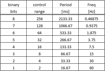
Because the ATmega328P master clock operates at 16MHz and the maximum TIMER2 divisor is 1024, the minimum PWM sampling frequency is ~30Hz yielding 4 levels of resolution control.  However if we further divide the ATmega328P master clock frequency by 8, then  PWM frequency is 3.75Hz with 5 bit (32 level resolution) is achieved.

Considering many practical applications, a sampling rate of ~4Hz with 5 bit resolution was an acceptable trade-off.  Implementing both TIMER2 pre-scalar 1024 and master clock divisor 8 is required to reach a PWM frequency of 16MHz/(1024*256*8*2) = 3.83 Hz. The master clock was divided in software with the clock_prescale_set(clock_div_8); instruction which of course has a similar affect on the delay(); instruction and delay values must be divided proportionally. The Arduino standard PID_v1 library was also edited for the same reason and a modified PID_v1R library is included in zip archive link below.

Testing
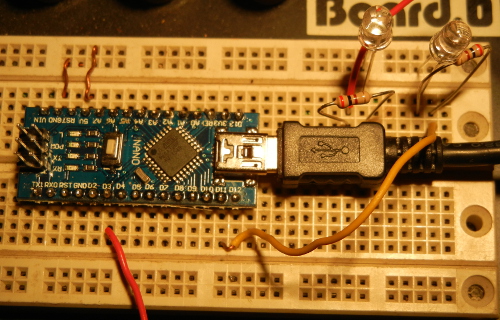
To debug and validate this design an Arduino Nano and breadboard was used with 2 LEDs, SSR and 60W incandescent light bulb. It was easy to see the LEDs flash at a slow rate (PWM cycle time) and the LED brightness change (PWM duty-cycle). The definitive test was using an SSR to switch a 120V resistive load (60W light bulb) and to my joy, flashing and variable brightness was observed. This was the extent of testing.

Arduino Nano Test Platform

Discussion
This was a satisfying project because I learned a lot about PID and made a practical PID temperature control unit for very cheap ($20). Almost all the Arduino I/O pins are used and SSR-PWM problems were overcome to a reasonable degree. Adding a menu structure to edit run-time variables from the existing keypad would approach the functionality of a real commercial unit. Adding timer functions could create temperature profiles and recipes(EEPROM). Some practical applications might include a Rice Cooker, Slow Cooker, alcohol fermentation. Some day I’m going to turn the PID problem around and make a device that senses meat temperature and indicates the remaining cooking time. Mom’s Thanksgiving turkey will be cooked perfectly every time.

References
Arduino_PID_Temp_Control_Program.zip
Wikipedia PID
SSR Types

MongoDB C100DBA Exam Study Guide

mongodb_logo_300x100Today I completed my MongoDB C100DBA database administration certificate exam. This proctored exam is taken remotely online through Examity. The exam session duration was 90 minutes which consisted of 60 multiple choice and all-that-apply questions. The way I study is to condense a summary of my knowledge into a single document. Just the act of writing coherent paragraphs about a subject aids in my memory and understanding. For this purpose I prepared MongoDB_C100DBA_Exam_Study_Guide

This study guide expands on topics referenced in MongoDB’s own C100DBA study guide, and the MongoDB online documentation. My exam was related to database v3.2.  I passed my exam and my certificate license is #295-0761-259.

In my opinion, the exam is rather difficult, requiring deeper knowledge and practical experience than what is nominally presented in M102, M202 online courses. Of course the good student will expand on these introductory courses and establish a working platform to explore the syntax, properties and exceptions of CRUD, indexes, replication, sharding, administration etc. of various possible test cases.

This guide is especially recommended for M102 students to find condensed detail notes and documentation links on this subject.

In PDF format, 35 pages. A_MongoDB_DBA_Exam_Study_Guide

J Pole Antenna SWR Tuning

For the DIY Amateur Radio enthusiast, few things in life are as satisfying as designing, building and testing your own homemade radio antenna. A 2 meter J pole antenna, constructed of 1/2″ copper tubing, is easy and cheap to make and almost guarantees practical success. With simple modifications, and careful SWR measurements, I was able to improve my j pole antenna swr performance.

diagram
Jpole Design

Many online web sites provide help on designing a 2 meter J-pole antenna and almost all designs are very close in configuration and dimensions (see References) which yield confidence for success. The 10 foot copper length of 1/2″ tubing and plumbing fittings cost $25 at the Home Depot store.  The SO-239 connector  was obtained from a local Surplus Electronics store for $3.50.  For cutting the Cu tubing lengths, I marked a wooden “Story Stick” for possible reproductions. Using propane torch, solder flux and solder, the antenna with connector was assembled.

so-239
Connector, SO-239

My new antenna seemed to work fine. But, in spite of my best accurate construction techniques, when I tested the assembled antenna, the SWR was too high (>3)  at the 148 MHz end of the 2m band. So I decided to modify the main pole and j-pole tips with adjustable screws. Turning the screws tunes the effective electrical length.

screw
Brass 6×32 Tuning Screw

To my delight I found that adjusting the screws would control the SWR, at least within a small range, I turned the screws to tune for the lowest SWR in the middle of the 2m band range (146 MHz).  My modified antenna works very well Tx and Rx. The improved SWR profile (shown below)  is attributed to screw modification and careful SWR tuning. I was satisfied with the screw modifications.

SWR
J-pole SWR (before and after tuning)


References:
Hamuniverse
Ceca

Rifle Ballistics Calculator

I grew up with a boy’s natural curiosity about Firearms. Considering to purchase Firearms, I searched for a way to compare and contrast ballistic characteristics from the wide variety of calibers available. Once I began to shoot, I wanted to sight a gun for accuracy. At last I found a complete computer rifle ballistics calculator program (technically, G1 projectiles). Not only was this program adaptable to a personal computer but it was developed by a career U.S. military ballistics researcher. Furthermore the calculation method relies on empirical results rather than heavy theoretical considerations often associated with fluid dynamics. After programming these routines I referenced manufacturer’s ammunition ballistic data and found a high degree of correlation with bullet velocity at range. This gave me confidence to develop a general ballistic application. I created the following webpage to graphically show ballistic results.

Renegade Rifle Ballistics

To use the webpage, the user begins by entering a name for their rifle load, then enters several initial ballistic quantities related to their ammunition (muzzle velocity, bullet weight, bullet ballistic coefficient), their firearm (scope/sight height) and environmental conditions (temperature, altitude). The user can also compare their load to one or more common firearm calibers.

One of the more difficult required entry quantities is the bullet ballistic coefficient. This coefficient is a measure of the bullet’s ability to resist the de-accelerating forces of air resistance. Physically, ballistic coefficient is related to bullet diameter, shape (cross section) and mass (weight). The larger the coefficient value, the longer/farther the bullet retains its velocity and energy. Ammunition manufacturers often publish this value and these values can be found online. Typically any caliber ammunition can be loaded with a variety of bullet types and coefficients, so careful selection is required. If a bullet coefficient cannot be found, the coefficient can be calculated using the link below. Enter 2 velocity, range data pairs from the manufacturer’s data. The most most accurate results can be obtained by measuring bullet velocity at 2 ranges using a chronometer.

Bullet Ballistic Coefficient Calculator

Ballistics Output

After clicking the “Fire” button, several graphs display the ballistic results (Trajectory, Kinetic Energy, Velocity and Time of Flight). As always, the trajectory of the bullet is exactly on target at the range specified by user input. An example plot is shown below.

Renegade Rfile Ballistics Trajectory Plot
Trajectory Plot for 3 common Calibers

Also on this page is a link to a custom target created from the user’s input data. An example target is shown below.

7mm Sighting Target
Custom Sighting Target

This target is in PDF format and can be printed on normal 8.5×11″ paper. To sight a rifle, mount the target at 100 yds. distance and aim for the center circle. The horizontal arrows indicate the impact point at various ranges. Adjust your sights in order to impact the line at the desired range. In other words if you want the bullet to be on-target at 200 yds. aim for the center and adjust your sights until the bullet impacts to 200 yd. horizontal line (slightly above the 100 yd. line). The horizontal range of the arrows shows the +/-3″ accuracy at each corresponding range.

Use the Renegade Rifle Ballistics webpage to advance your shooting ability.

US Amateur Radio Callsign Query

Antenna
World-Wide Communications

After upgrading my Amateur Radio license class from General to Amateur Extra, I contemplated applying for a Vanity Callsign. But what Callsigns were available to me? For amateur radio operators, Callsigns are as personal as names and I wanted something special. After searching online I couldn’t find a website or webpage that really showed, in a concise manner, available Callsigns. So, I created the webpage noted by the link below.

US Amateur Radio Callsign Query

The main table is arranged by license class, format, region code that helps the user find appropriate Callsigns fast. Of course competition for the most exclusive Callsigns is fierce but you may want a Vanity Callsign that reflects your name, or your Amateur Radio Club name or location. Refer to the FCC (Federal Communications Commission) website for Vanity Callsign eligibility and application process. For example, an Amateur Extra class license holder is eligible for just about any available Callsign without regard to region or other license classes. The ARRL (Amateur Radio Relay League) website offers a concise explanation regarding Vanity Callsigns.

Here, available Callsigns are sourced from publicly-available data at the FCC. It is automatically updated every week (Sunday midnight). So the best time to reference new data is every Monday morning. The FCC website allows you query information about the status of particular Callsigns. According to FCC regulation 97.19(2), cancelled callsigns are available 2 years after the cancellation date. This is often different from the official expired date displayed at the FCC license search. Use the available_date shown here to find your callsign. Only callsigns existing within the FCC’s ULS are shown here. Many callsigns are yet to be assigned, or sequential gaps exist. Verify callsign availability at the FCC website. Submit an online or written application and fee.

Please direct your comments, questions to kf7gax(@)arrl.net

$20 VHF 50 Ohm Dummy Load

As a HAM Radio enthusiast I like to think I can design, build and evaluate RF Antennas. To help me calibrate my SWR meter I decided to build a VHF 50 ohm dummy load. Naturally, an ideal dummy load  is purely resistive (no reactive component).

I visited my local Electronics Surplus Store to purchase a 50 Ohm, thin film Beryllium Oxide (BeO) resistive load. Ceramic wire-wound  resistors were cheaper but they react more like RF inductors. In general, BeO loads are rated for 3-20GHz and 5-200W, but of course we must never exceed the max rated temperature, 100C (?), so a Heatsink is required. My surplus shop also sold an SO-239 panel mount connector. This is a common VHF/UHF (0-300MHz) connector used in radio communications. Resistor, connector and heatsink component cost was about $15.

VHF Dummy Load
Front View note: SO-239 Connector

The heatsink is resourced from an SSR (Solid State Relay). SSRs are rated for 40W continuous. Be careful. Watch the temperature! A nearby fan may marginally cool. A flexible thermal pad is installed between resistor body and heatsink for better thermal contact.

Side View
Side View

To complete the ground circuit, 14 gauge multi-strand wire is soldered to  resistor coax shield and PCB (and SO-239 connector shield). Luckily the resistor shield was not Aluminum.

back
Ground Connection

I tested this with my 75W 2 meter ham radio rig. Works well but at full power it gets hot in a few seconds. I’ll use this load to calibrate my SWR meter readings.

Load50-SWR
SWR ranges from 1.0 to 1.3 at 300MHz max freq.

Using a Network Analyzer, I gathered performance data over the frequency range of 0 – 300 MHz. Above is shown Standing Wave Ratio plot. SWR ranges from 1.0 (ideal) to 1.3 (good) at max frequency.

Smith Chart
Impedance barely deviates from 50 ideal resistor over frequency range

Smith Chart above shows that the load impedance (blue curly-q) is close to ideal 50 ohm resistance over the frequency range.

Load50_TDR_553In this Time Domain Reflectometry (TDR) plot  the grossly soldered connector is obvious as it ranges from 30 to 80 ohms near the connector. Nevertheless the performance at lower frequency is OK.

Wood Fence Repair

After 23+ years the wood fence in the side yard collapsed.  The posts had rotted at ground level and the fence fell over against the house.

Collapsed Fence
Collapsed Fence

2 old fence posts were dug out of the ground and replaced using 4x4x8ft pressure treated wood posts and an 80lb. bag of Quikrete.

Concreted Posts
Concreted Posts

Pressure treated 2×4 rail attached using galvanized metal hanger. Cedar stile joined with 1.25″ deck screws. The material cost was about $60 per 8 foot section.

Construction Detail
Construction Detail

The repaired fence standing tall and proud.

repaired fence
Repaired Fence

Repaired fence viewed from neighbor’s yard

neighbor's fence
Neighbor’s Fence

Canning Appliance

Recently I toured a farm’s harvest processing facilities and mentioned to the farmer that I thought I could automate one of his processes. He challenged me to build such an appliance, so I did.

Using a commercial 1500W hotplate and an Omega temperature controller I fabricated the appliance shown below. A Solid State Relay (SSR) switches power to the hotplate to modulate temperature. The controller operates in four modes (temperature display, constant temperature and ramp/soak program, PID). Since the hot plate operates only in on/off mode I couldn’t use the PID (Proportional Integral Differential) mode.

Front view testing
Front view testing


Top View
Top View


More Testing
More Testing


Wiring in Bottom
Wiring in Bottom


After using my canning appliance, the happy farmer reported that he was able to control temperature within a +/- 3F range. And this resulted in shortened process times and more uniform product.

Download Design Docs in PDF Format

A Wood Sign

I made this wood sign for my sister to display on her farm.

The letters are cut into a 1×8″ red oak dimensioned lumber board using a hand-held plunge router and Rockler’s 3.5″ State Park font  templates. This style includes Kerning, an attractive way to space certain letter combinations. The letters are painted black and the board is finished with shellac and several coats of polyurethane.

wood sign
Sign at the Farm


wood sign
Sign Close-up


 Rockler State Park Font Kit

Drop Leaf Gate Leg Folding Oak Table

I made this gate leg drop leaf table based on a design from MLCS Industries. plans here.

A critical feature is the Rule Joint that allows the leafs to fold down but support weight when the leaf is up.  The Rule Joint also requires a special metal hinge and mortising on the table under side.  The Rule Joint was carved into the table top using a hand-held router and 2 simple router bits. The table apron is formed with mortise and tenon joints plus metal clasps (not in the plans). All wood is white oak, stained with Minwax oak and protected with multiple coats of polyurethane. I spent a lot of time flattening the top surface with a card scraper.

side view
side view: gate leg and leaf fold together precisely
leafs folded
leafs folded


half open
half open


fully open
fully open: lots of table space


Strong and tough, this table is one of my most successful woodworking projects and is in daily use at my niece’s home. The MLCS plans make an attractive gate leg drop leaf table.